How can I fix regression model interpretation of feature?

Question

I'm building a regression model to predict the values of a feature $Y$ given a set of other features $X_{1}, X_{2}, X_{3}..X_{n}$.

Onde of these other features, let's say $X_1$, is known to be inversely proportional to $Y$ based on domain's knowledge. The problem is my model is interpreting his coefficient as positive, letting it directly proportional to $Y$. I've tried plenty of different models to verify if I could get better interpretation, such as OLS, Linear Regression, and Logistic Regression, but every model I tried failed to interpret the $X_1$ coefficient.

What can I do to get a regression that better reflects the real-world behavior of this coefficient?

so u expect the coef of X1 to be negative because it is inversely proportional to Y? — develarist, Apr 27 '20 at 22:26
What exactly do you mean by "$X_1$ is known to be inversely proportional to $Y$"? Univariate analysis, domain knowledge, theoretical fact, ...? — Ben Reiniger, Apr 28 '20 at 02:15
It's only domain knowledge. I'm working on a model to make some prediction scenarios. One of these scenarios consists of raising the values of $X_{1}$. I expect $Y$ to go down, but $Y$ raises too, which in the domain of the features is wrong behaviour. — Tiago Bachiega de Almeida, Apr 28 '20 at 02:31

score 5 · Accepted Answer · answered Apr 28 '20 at 05:07

Unless there's a mistake in your code, or the coefficient on $X_1$ is not significant, I'd be inclined to trust the model output.

It's not unusual for data to behave this way. Just because $X_1$ and $Y$ are inversely related with respect to the marginal distribution of $(X_1, Y)$, as can be concluded from a scatterplot of the two variables, does not mean this relationship holds conditional on other variables.

Here is an example where $(X_1, Y)$ are inversely related, but are positively related conditional on another value, $X_2$. (The example is generated using R -- you've tagged python, but this concept is language-agnostic):

library(tidyverse)
library(broom)
set.seed(1)
N <- 100
dat <- tibble(
    x2 = sample(1:4, size = N, replace = TRUE),
    x1 = x2 + rnorm(N) / 3,
    y = x1 - 2 * x2 + rnorm(N) / 5
)
ggplot(dat, aes(x1, y)) +
    geom_point(aes(colour = factor(x2))) +
    theme_bw() +
    scale_colour_discrete("x2")

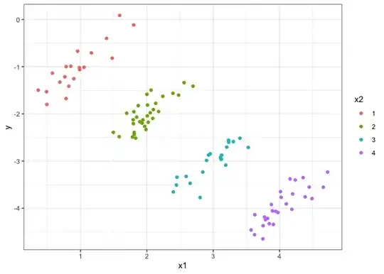
Here are the outputs of a linear regression model. You'll notice that the coefficient on $X_1$ is negative when $X_2$ is not involved, as anticipated, but is positive when $X_2$ is involved. That's because the interpretation of a regression coefficient is the relationship given the other covariates.

lm(y ~ x1, data = dat) %>% 
    tidy()
#> # A tibble: 2 x 5
#>   term        estimate std.error statistic  p.value
#>   <chr>          <dbl>     <dbl>     <dbl>    <dbl>
#> 1 (Intercept)   -0.492    0.154      -3.20 1.83e- 3
#> 2 x1            -0.809    0.0549    -14.7  1.33e-26
lm(y ~ x1 + x2, data = dat) %>% 
    tidy()
#> # A tibble: 3 x 5
#>   term        estimate std.error statistic  p.value
#>   <chr>          <dbl>     <dbl>     <dbl>    <dbl>
#> 1 (Intercept)   0.0189    0.0540     0.349 7.28e- 1
#> 2 x1            1.04      0.0681    15.3   1.42e-27
#> 3 x2           -2.05      0.0726   -28.2   1.60e-48

^{Created on 2020-04-27 by the reprex package (v0.3.0)}

This concept extends to more than two covariates, as well as continuous covariates.

Thanks for the enlightening answer. I will give a better look for the other features and verify how can I better use then to get the expected results. — Tiago Bachiega de Almeida, Apr 28 '20 at 12:30

score 0 · Answer 2 · answered Apr 29 '20 at 09:56

The model can only see the data provided for training. Not the domain truth.

1. Is your Y inversely proportional to X1
- Check with a simple scatterplot
- Also, try to see the correlation strength(with Y) with a correlation matrix

2. If No,
- Check the data source and understand the conflict

3. if Yes,
Possible cause can be the impact of any other variable(pointed in the accepted answer), you can try these -

- Forward selection, build a model with X1 and see the coef_, must be -ve and then add other variables one by one and see which variable does this
- Check the Correlation with other variables, X1 might be a less important feature. This might give you a new insight to look into in your data and domain

How can I fix regression model interpretation of feature?

2 Answers2