Elimination of features based on high covariance without affecting performance?

Question

I ran into a question where the answer ran me into a big doubt.

Suppose we have a dataset $A=${$x1,x2,y$} in which $x1$ and $x2$ are our features and $y$ is the label.

Also, suppose that the covariance matrix between these three random variables are as follows:

$$\begin{array}{|c|c|c|} \hline &x1&x2&y\\ \hline x1&a&d&e\\ \hline x2&d&b&f\\\hline y&e&f&c\\\hline \end{array}$$

When $|d| \gg 0$, someone may ignore either of the two features, without losing any performance.

The claim was marked as a true question. Is there any idea why the mentioned proposition is True and performance was not affected?

Answer 1

$|d| \gg 0$ means there is a very strong correlation between $x_1$ and $x_2$. This means one can be expressed (almost completely) in terms of the other, thus one of two is almost redundant.

A simple example:

Consider that $x_2$ is simply a copy of $x_1$, ie $x_2=x_1$. Does $x_2$ offer any new information about the the label $y$ apart from the information $x_1$ provides? No, it is clear.

Now consider that $x_2$ is simply a shifted version of $x_1$, ie $x_2=c_0+x_1$. Does it now offer any new information apart from what $x_1$ provides? Again no, by simply changing the reference point $c_0$, which is equivalent to changing the baseline of the measuring system, does not by itself offer new information.

Thirdly consider that $x_2$ is a re-scaled version of $x_1$, ie $x_2 = s \cdot x_1$. Does it offer now different information than what $x_1$ provides? Again, no since scaling is equivalent to changing the measuring unit of $x_1$, but this is simply a re-naming of units, no new information is added.

One can see that any transformation of the form $x_2 = c_0 + s \cdot x_1$ does not offer any new information from what $x_1$ already provides, by the arguments above.

If one wants to be more realistic one can add some noise, ie $x_2 = c_0 + s \cdot x_1 + \epsilon$, where $\epsilon$ is some random variable with zero mean and very small variance.

A correlation value $|d|$ which is quite high actualy means that $x_2$ can be expressed as such a transformation of $x_1$, ie $x_2 = c_0 + s \cdot x_1 + \epsilon$ (or vice-versa) (there are some non-trivial exceptions to this). So $x_2$ offers no new information apart from what $x_1$ offers and is redundant.

So if such a high correlation exists between variables/features, one of them can be always eliminated without diminishing performance as being redundant (in the sense that, as far as second-order statistics are concerned, the two variables are identical).

This is one of the main rationales of feature selection and dimensionality reduction in machine learning.

Answer 2

I primarily agree with @NikosM., but take issue with the question's assertion (my emphasis)

without losing any performance

Having very high correlation means they are very nearly in a linear relationship, but it is possible that the deviation from linearity is not random, and in fact is predictive. Here's a simple example:

import numpy as np
import matplotlib.pyplot as plt
from sklearn.linear_model import LinearRegression
from sklearn.model_selection import cross_val_score, KFold

x1 = np.linspace(0, 10, num=1000)
x2 = x1 + np.sqrt(x1)
X = np.vstack([x1, x2]).T
y = np.sqrt(x1)  # so y = x2 - x1

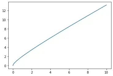
plt.plot(x1, x2);

print(np.corrcoef(x1, x2))  # = 0.9991

lr = LinearRegression()
cv = KFold(shuffle=True, random_state=314)

print(cross_val_score(lr, X, y, cv=cv).mean())
print(cross_val_score(lr, x1.reshape(-1,1), y, cv=cv).mean())
print(cross_val_score(lr, x2.reshape(-1,1), y, cv=cv).mean())

outputs

1.0
0.9592797987922872
0.9741089428341769

and the plot of $x_1$ vs $x_2$: