Disclaimer: Even though I posted a relevant link (in a comment to the question ) which can answer the exact question asked, I am not familiar enough with continuum mechanics to actually explain it. Having said that ...
The behavior seen in continuous elastic material may have discrete spring mass analogues.
Qualitative / by Analogy
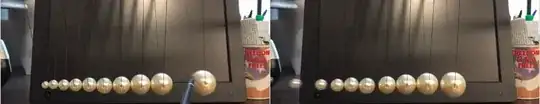
Consider a Newton's cradle. All the balls are identical. You input a specific displacement to a ball at one end. That ball then drops and collides with the rest. The energy is transferred to the ball at the other end which is identical and so moves by the same amount.
Now consider a case where the balls are non identical. The displacement can be larger or smaller depending on mass of the last (and perhaps intermediate) ball. If the last ball is smaller, it will under go a larger displacement than the ball on the input side.
- Galilean cannon.
- A video showing different ball sizes (dur : 3:33).
- Newton's cradle with varying ball size (dur : 2:21)
The oscillations in an ultrasonic horn are linear in nature and the above examples involves collisions (non linear ?); so the logic may not carry over one-to-one. The basic ideas of energy transfer and energy conservation still apply.
If this logic carries over to the ultrasonic horn, then a smaller end would be expected to under go larger displacement since a smaller cross section would need to compress/expand by larger amount when forced to store the same (elastic) energy that was supplied at the input.
But, A short search of literature clearly shows that ultrasonic horns can have diverging sections also; apart from converging sections. Examples seen in literature show horns having multiple converging-cylindrical-diverging section. This may be due to other reasons and may not invalidate the above explanation. So the discrete analog of the system may not be a perfect analogy.
(kind of) Quantitative
The one dimensional partial differential equation can be discretised in spatial domain. The equation given in the linked reference literature is
$$
\frac{\partial }{\partial x}(S\cdot E \frac{\partial u}{\partial x}) dx
= S\cdot \rho \frac{\partial^2 u}{\partial t^2} dx
$$
On discretising, the RHS becomes $m_i \frac{d^2 u_i}{d t^2}$ where $m_i$ is the ith discrete mass.
On the LHS, the $\frac{\partial^2 u}{\partial x^2}$ will take the form $u_{i+1}+u_{i-1}-2u_{i}$ and $ \frac{\partial S}{\partial x} \frac{\partial u}{\partial x}$ will take the form $p\cdot (u_{i+1}-u_{i})$ where $p$ depends on the taper and $p=0$ for the cylindrical section.
So the discretised equation will be of the form
$$
a u_{i+1} -b u_{i} + c u_{i-1} = \frac{d^2 u_{i}}{d t^2}
$$
The eigen vectors of this discretised system will provide the deflection at resonance.
An Octave code which attempts to construct the system and then find its eigen vectors is given below. (code is not verified; doesn't follow physical units)
  clc;

  % number of elements / sections
  n = 100;

  choice = 3;

  switch(choice)
    case 1
      % cylindrical section
      si = ones(1, n);
      tstr = 'cylinder';
    case 2
      % linear taper
      si = linspace(10, 1, n);
      tstr = 'linear taper';
    case 3
      % step at half length
      si = [10*ones(1, n/2), 1*ones(1, n/2)];
      tstr = 'step';
  end

  % normalize area so that
  % the net mass is the same for each case
  si = si/sum(si);

  % mass proportional to area. density = 1
  mi = si;

  sum(mi) % check mass

  % spring constant of spring from ith to i+1th section
  % spring constant proportional to average area of neighboring sections
  ki_ip1 = (si(1:end-1) + si(2:end))/2;

  %% differential equation
  % M xdd = K x
  % xdd = M^-1 K x;

  M = diag(mi);

  K = diag(ki_ip1, 1) ...   connection to m_i+1
     +diag(ki_ip1, -1) ...  connection to m_i-1
     -diag([ki_ip1, 0]) ... connection of other end of spring m_i
     -diag([0, ki_ip1]);... connection of other end of spring m_i

  % attach the first node "rigidly" to wall
  % if boundary condition requires it
  % but the paper states the "free-free" assumption instead.
  % K(1,1) = K(1,1) - 100;

  % find the mode shapes of M^-1 K
  A = -M\K;
  [V, lambda] = eig(A);

  % normalize the input end to +-1
  % this allows us to see the "amplification" at the free end
  % for various rod shapes
  V = V ./ repmat(V(1, :), [n, 1]);

  % normalize the "free" output end to positive value
  V = V .* repmat(sign(V(end, :)), [n, 1]);

  % extract the square of the frequency
  lambda = diag(lambda);

  % sort by frequency
  [l, iii] = sort(lambda);

  % plot mode shape low freq modes
  % the second mode is the important mode to note.
  figure(1);
  select = 1:4;
  plot(V(:, iii(select)), 'linewidth', 1.5);

  legend(num2str(sqrt(l(select))), 'location', 'northwest');
  title(tstr, 'fontsize', 14);
  set(gca, 'fontsize', 14);
  xlabel('node number');
  ylabel('normalised amplitude');
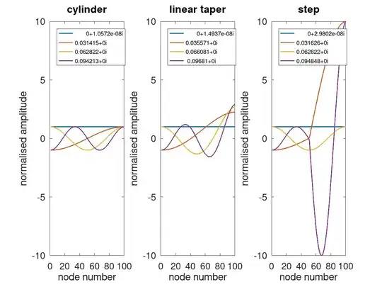
The resulting mode shapes (first 4 modes including 0 frequency mode) from above code is shown below. As mentioned in the linked paper, mode shapes for the cylindrical horn are sinusoids. Mode shapes for the stepped horn are sinusoids of differing amplitudes.
Both the converging shapes show amplification at the free end when compared to the cylindrical horn.
Quantitative
Extracting the mode shapes from a proper FEM model will give the free end amplification for complicated shapes.


