Thermal plumes have been studied extensively for fire safety applications. Often you know the heat release rate $Q$ but little more. A dimensionless group called $Q^*$ (pronounced "Q star") is used instead of more common parameters like the Reynolds number and Rayleigh number. This parameter can be thought of as the strength of the heat source at a particular distance. It correlates well for thermal plumes. You can derive this group by non-dimensionalizing the Navier-Stokes equations and setting dimensionless groups equal to 1 to define the characteristic length and velocity. For more information, check out Gunnar Heskestad's paper on this dimensionless group.
In the fire modeling case, generally people ignore Prandtl number similarity and some other things, so they say the dimensionless temperature and velocity distributions are only functions of $Q^*$.
The most relevant parameters are:
$$T^* \equiv \frac{T - T_\infty}{T_\infty}$$
$$Q^* \equiv \frac{Q}{\rho c_p T_\infty (g x)^{1/2} x^2}$$
To be more explicit, if you know the temperature ($T$) as a function of height ($x$) above the hot object, you can find $T^*$ as a function of $Q^*$. $Q^*$ is like a dimensionless spatial coordinate.
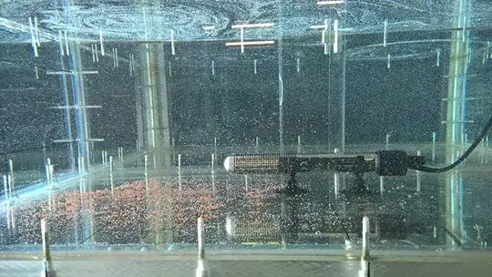
Strictly speaking, your setup is not going to be exactly similar because your coil and a human are not geometrically similar (and the heat flux distribution on the coil is probably not similar either). In your photo, I assume the human would be lying down if any reasonable geometric similarity is desired. The far-field should be okay, and I'll assume this is what interests you [2].
It's also not exactly clear what quantity you are interested in. I assumed you want to get the temperature distribution in the plume, say, at a height $x_1$ above in reality which would be $x_2$ in your model. Correct me if this is wrong.
Also, while I don't do experiments, I imagined your heating coil has an output of $W$, not heat flux. Let me know if I'm mistaken and I'll change my answer.
Ignoring the other parameters may or may not be valid in your case (it seems to be okay for fire safety [1]), so I'll do the analysis assuming it's not. You can skip the remainder if you want to assume the two mentioned parameters are all you need.
You can get the number of required groups from the Buckingham $\pi$ theorem.
The relevant parameters I've identified are $T$ (temperature at height $x$), $x$, $Q$, $g$, $\alpha$, $\beta$, $\nu$, $T_\infty$, $\rho$, and $c_p$. The Buckingham $\pi$ theorem suggests there will be 6 dimensionless groups here. (Assuming that I am not missing a parameter. I also need to check that the dimensional matrix is not rank deficient. For more details about dimensional analysis, I recommend reading Dimensional Analysis and Theory of Models by Henry Langhaar.)
So, the first 5 dimensionless groups are:
$$T^* \equiv \frac{T - T_\infty}{T_\infty}$$
$$Q^* \equiv \frac{Q}{\rho c_p T_\infty (g x)^{1/2} x^2}$$
$$Pr \equiv \frac{\nu}{\alpha}$$
$$Gr_x \equiv \frac{g \beta (T - T_\infty) x^3}{\nu^2}$$
$$\rho^* \equiv \beta (T - T_\infty)$$
This fifth group is inspired by the Boussinesq approximation. In that approximation, the density difference is modeled as a temperature difference. Similarity in this parameter ensures that your density field is similar.
For the remaining group, I needed to get a little creative. Similarity does not require this group takes any particular form, but it's best to stick with parameters with known physical meanings (or parameters which can be derived from governing equations, which usually have physical meanings). I can't think of anything good off hand, but the following works:
$$\Pi_6 \equiv \frac{g x}{c_p(T - T_\infty)}$$
You need to match all of these for similarity. It should be clear that matching all of these will be a challenge. As I said, it appears to be common practice in fire safety to ignore everything but $T^*$ and $Q^*$. I don't know if this is because the other parameters don't matter, or if it's just for convenience. Sorry if this is not the answer you expected, but as with many things in engineering, the answer is not easy.
[1] I remembered later that the non-dimensionalization of the Navier-Stokes equations suggests that $Q^*$ is the only parameter in the solution. So perhaps $T^*$ and $Q^*$ are all you need, and the Buckingham $\pi$ approach just gives you superfluous parameters. I don't recall all the details of the non-dimensionalization, but if there is interest I'm sure I could reproduce it.
[2] The theoretical argument that supports the use of $Q^*$ assumes the heat source is a point source. So it's really only correct far away, because the temperature goes to infinity at the point source in the model. This is because $Q^*$ goes to infinity at $x = 0$, as you can see from its definition. If you are developing a correlation, say $T^* = a (Q^*)^b$ where $a$ and $b$ are coefficients, you can get around this by defining a "virtual origin", which will allow you to develop a correlation without singularities. Basically, instead of using $x$ you define use instead $x_\text{virtual} = x + x_\text{origin}$. That is, $Q^*$ is now written:
$$Q^* \equiv \frac{Q}{\rho c_p T_\infty (g [x + x_\text{origin}])^{1/2} (x + x_\text{origin})^2}$$
You pick $x_\text{origin}$ such that your correlation fits better. It's another parameter in the correlation. If you know the surface temperature, you can pick $x_\text{origin}$ such that the surface temperature is what the correlation returns at $x = 0$.
Also, as the argument supporting the use of $Q^*$ really makes the far-field assumption from the beginning, it's not clear that simply using a virtual origin is enough to make a correlation valid in the near-field (even if you have geometric similarity). I can't say whether or not the other factors I've identified factor in or not.